By Vasyl Postolovskyi and Olle Gladso
Contributing Writers and Instructors at Riverland Technical and Community College in Albert Lea, MN
In Part 1 of this Maximizing Tools series, we discussed an alternative approach to diagnosing an engine using the pressure waveforms from an in-cylinder pressure transducer. Part 2 continues our discussion in more detail, analyzing the Valve Timing and Ignition Timing tabs on the waveforms. Part 3, which will be featured in our October/November issue, will discuss the Inlet (or Intake) and Exhaust tabs. To view Part 1, see the April/May 2014 edition or visit http://bit.ly/StA6pi.
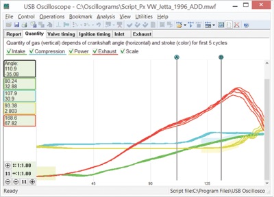
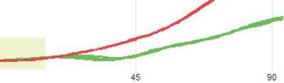
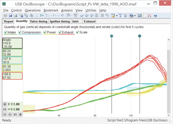
As can be seen in Figures 1 and 1a, with late cam timing, the red and green traces — showing exhaust and intake gas volume, respectively — overlap for the first approximately 20-30° of crankshaft rotation away from TDC.
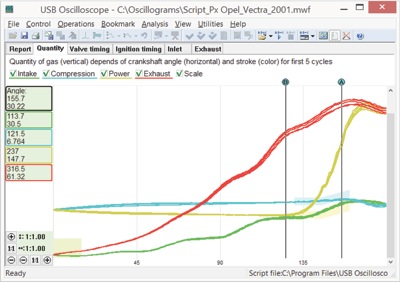
If the camshaft is installed one tooth early, the valve timing is advanced. This is the same as early opening and closing of the valves. In Figures 2 and 3, that is shown as an offset of the closing of the intake valve to the right, and opening of the intake valve to the left. Again, the characteristic points are moving away from each other approximately 30°.
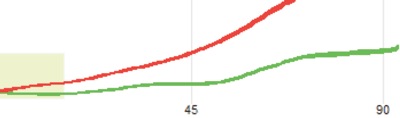
The waveform distortion shown in Figure 3, where the valves are overlapping, is typical for advanced valve timing. The red and green traces do not overlap each other as they did with late valve timing and they have characteristic angles.
On engines equipped with a chain-driven camshaft, the shift of the opening and closing valves becomes larger than on engines equipped with a timing belt.
We have shown that valve timing can be quickly and accurately analyzed and verified using the method described.
The “Valve Timing” Tab
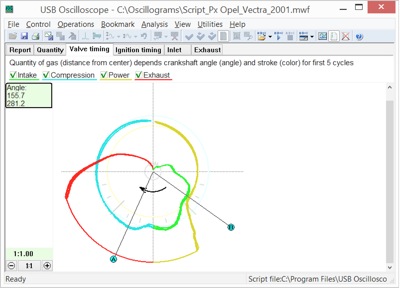
This tab provides a diagram that gives the same information about the volume of gas in the cylinder as the “Quantity” tab does, but shown in relation to the angle of the crankshaft. The amount of gas in the cylinder is expressed as the distance from the center of the diagram. The trace’s distance from the center is a visual representation of the amount of gas in the cylinder.
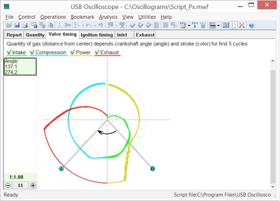
Figure 4, which is a polar diagram, shows the amount of gas in the cylinder depending on the angle of the crankshaft and the stroke of the tested cylinder. The A marker shows where the intake valve is closed, and the B marker shows when the exhaust valve begins to open. Note that the marker locations are symmetrical relative to the vertical line.
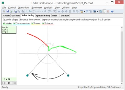
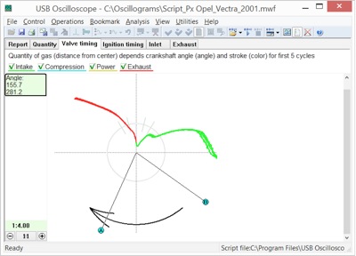
Figure 5 is a zoomed in capture showing more detail on the center of the diagram from a typical engine in good working order.
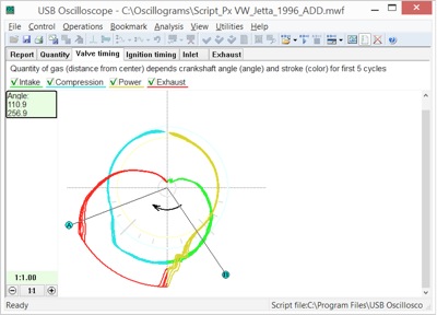
If the timing belt or chain is installed one tooth late on engines equipped with a single camshaft, the valve timing for both intake and exhaust will be late. On the polar diagram, this shows as a rotation of the valve phase diagram clockwise about 15° (if there’s a timing belt; more if there’s a chain). The intake valve closing and the exhaust valve opening are no longer symmetrical relative to the center line or TDC. This asymmetry is shown in Figure 6. The late valve timing also manifests as a distortion in the center of the diagram, as shown in the zoomed-in diagram in Figure 7.
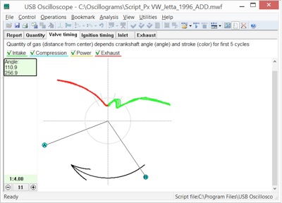
The first phase of the distortion in Figure 7 occurs because the piston, after passing TDC in the cylinder, starts to create low pressure in the cylinder and gases will flow from the exhaust manifold through the still-open exhaust valve. The second part of the distortion occurs because the piston is already on its way down in the cylinder when the intake valve opens.
If the timing belt or chain is installed a tooth early, the valve timing will be advanced and the polar diagram will again be asymmetrical. Under this condition, the diagram will be rotated counterclockwise. The valve phases shown in Figure 8 will again be asymmetrical relatively to the horizontal or TDC line. Figure 9, which is a zoomed in part of Figure 8, shows distortion in the center. Note that the distortion looks different from what it does with late valve timing.
The distortion of the red trace on the diagram in Figure 9 is due to gases from the cylinder flowing into the intake manifold because the intake valve opens too early.
As is shown, the “Valve Timing” and the “Quantity” tabs can both be used to determine and diagnose valve timing issues. Which one to use is simply a matter of personal preference.
With some practice, these diagrams can be used with variable valve timing as well. If the diagram from an engine in good working order is known, variations due to timing belt, chain or cam phasers are readily apparent in the waveforms.
The “Ignition Timing” Tab
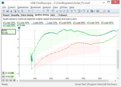
If a synch signal from a plug wire or similar was recorded along with the data from the pressure transducer, the Px script will also construct an ignition timing diagram, as shown in Figure 10.
In Figure 10, colors are used to signify the load on the engine with green being the lowest engine load and red the highest. Green is 20% load and red is 90% load. The higher the load, the warmer the color.
Normal operation of the ignition timing is shown in the diagram. As the engine rpm increases, so does the ignition timing. This is what used to be called centrifugal advance. On the diagram, this advance is shown as an increase in the graph height as we move toward higher rpm (to the right). Normal operation also implies that the ignition timing will vary with load on the engine.
With increasing cylinder pressure, also known as decreasing manifold vacuum, the ignition timing should delay, so the spark occurs later. The opposite is also true; with decreasing cylinder pressure, also known as increased manifold vacuum, the ignition should occur earlier, or advanced. Because the ignition is delayed with increased load, the red trace, which signifies high load, is located lower in the diagram than the green. The shaded areas signify where the ignition timing will normally occur. Events outside the shaded areas indicate malfunction.
When the engine in a modern vehicle is overrunning, as happens when you abruptly release the accelerator pedal or when the vehicle is decelerating, for example going downhill, the fuel supply is interrupted. Because there is no fuel supply in this mode, the ignition timing does not affect to the engine performance, so the corresponding traces on the diagram in this tab are not displayed by default.
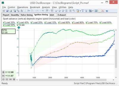
They can be turned on manually as is shown in Figure 11, and will display as blue traces. Blue signifies very little load. Note that the ignition timing is very late unless the engine is at very high rpm. This can be verified and proven with a timing light, if needed. Because the operating conditions are outside normal range (overrunning), the blue trace is slightly below what is considered normal range.
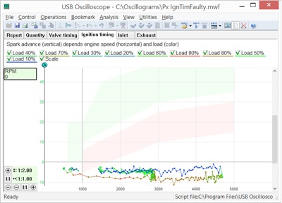
If there is a control or adjustment problem, the timing traces will appear outside the shaded areas, as is shown in Figure 12. In this example, the ignition timing is very late and does not adjust with either rpm or load. The engine will have very low power. This problem was caused by a faulty engine control unit.